[Artificial Intelligence] 01. Search (1): uninformed search

1. Agent와 관련된 기본 개념 정의

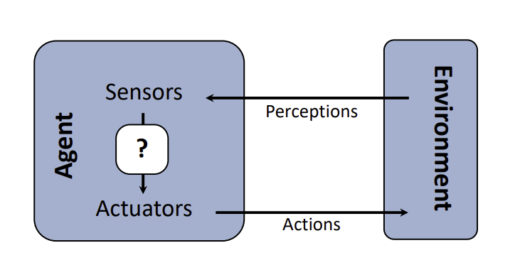
• Agent: 목표(goal)를 가진 개체(entity), 환경을 통해 얻은 perception에 근거하여 일련의 action을 취하는 존재
• Rational Agent: 합리적인 에이전트. 가장 기대되는 결과를 위한 행동을 선택하여 수행. 즉, 미래가 불확실하더라도, 가능한 모든 결과를 확률적으로 고려했을 때 자신에게 가장 큰 이득을 가져다줄 것이라고 계산되는 행동을 선택하여 수행함.
• Reflex Agent: naive한 agent, 선택하려는 행동이 미래에 어떤 결과를 가져다줄 지 계산하지 않고, 현재의 perception에 기반해 행동을 선택 및 수행. 1개 step만 고려함. Rational하다고 보기 힘듦.
• Planning Agent: what if. 행동의 결과에 기반해 결정을 내리는 에이전트. environment에서 시뮬레이션할 수 있는 능력이 필요함.
• Environment: 환경. 일반적으로 복잡함. (이유: 부분적으로 보임, stochastic(확률론적), multi-agent, dynamic, …)

2. Search Problems(탐색 문제)

탐색 문제의 구성 요소

• State(상태): 에이전트가 속한 환경의 모든 구성 요소들이 특정 시점에 배치된 완전한 상태
• State space(상태 공간): 에이전트가 마주할 수 있는 모든 가능한 state의 집합
• Start state: 탐색 문제를 해결할 때에 처음 시작하는 상태

• goal test: goal state로 가는지를 판단하는 함수
  cf. goal state는 여러 개일 수 있음

• Set of actions: 각 state에서 가능한 행동들의 집합
• Transition model(transition function, 전이 모델 또는 전이 함수): 특정한 action이 현재 상태에서 발생했을 때 다음 상태가 무엇인지를 도출하는 모델/함수

• action cost: 하나의 상태에서 다른 상태로 action과 함께 움직일 때 발생되는 비용
  cf. 그래프(또는 트리)에서 각 노드는 state로, edge는 action(정확히는 action에 의한 결과, transition)으로, action cost는 각 edge의 가중치로 표현됨.

• World state: 환경에 대한 모든 세부정보(detail)이 포함된 것(가장 객관적이고 완전한 환경)
• Search state: 모든 detail을 담고 탐색하는 것은 불필요하고, 불가능하기에, search 시에 필요한 key detail들만 필요
• Size of state space: 상태 공간의 크기. 탐색 문제를 푸는 computational runtime에 영향을 줌. 효율적으로 설계해야 함.

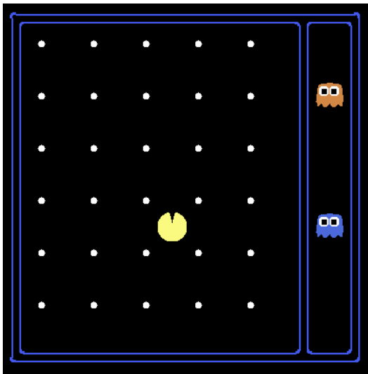
eg. 만약 다음과 같은 PacMan 게임이

• Agent position: 120 가지
• Food pellet count: 30 개
• Ghost positions: 12 개
• Agent facing: NSEW

다음과 같이 있다고 할 때, world state 개수는 $120 \times (2^{30}) \times (12^2) \times 4$ 이다.
이때, 단순히 Pathing 만을 위한 searching problem이라면, 120 가지의 world state를 상정하는 것이 옳다.
하지만, Eat-All-Dots. 즉, pellet을 모두 먹도록 하는 searching problem을 가정한다면, $120 \times 2^{30}$ 가지의 world state를 상정하는 것이 좋다.

3. Planning(계획) & Search Algorithms

State Space Graphs & Search Trees

1. State Space Graph => exact problem state가 노드
   searching problem을 수학적으로 나타낸 방식
   Node: 추상화된 world configuration. 즉, state
   Edge: transition을 표현(action에 대한 결과)
   
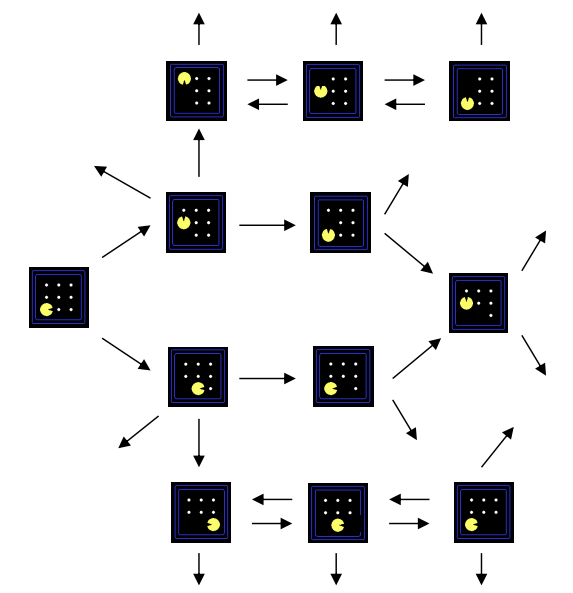
   각 state는 오직 한번 일어나며, 너무 커서 full graph를 메모리에 빌드하기 어려움
   따라서, 일반적으로 작은 search graph를 불러와 해결하는 아이디어는 유용함

2. Search Tree => plan이 노드
   what if tree of plans and their outcomes
   즉, 문제 자체의 구조가 아닌 문제의 해를 찾는 과정을 표현한 트리(cycle X)
   root node는 start state이고, 각 자식 노드들은 successor에 의해 정해짐.
   각 노드들이 state를 보여주긴 하지만, 각 state들이 달성하려는 plan에 대응함.

State space graph vs. Search tree

1. 노드 측면
   state space graph: 정확한 problem states. 문제 자체의 구조를 그래프로 표현한 것
   search tree: plan(state space graph 상의 전체 경로)을 나타냄
2. construction(구조) 측면
   둘 다 너무 커서 메모리에 빌드하기는 힘들지만, 가능한 작게 만들어야 함
   일반적으로, 탐색 문제에서는 search tree를 활용함
   이유: 목표에 도달하기까지 반복적으로 자식 노드들을 바꿔가며 당장 탐색하고 있는 상태들을 저장할 수 있음

Tree Search (DFS vs. BFS vs. UCS)

용어 및 과정 정리

• Frontier: 다음에 탐색할 후보 노드(state)들의 집합
• Search Process
  1. start state에서 시작
  2. partial plans의 outer frontier는 유지
  3. 선택된 노드를 제거하면서 frontier를 확장시키고, 모든 자식 노드들로 frontier를 교체
• 일반적인 frontier 탐색 전략(위에서 선택된 노드를 어떻게 고르는지)에 따른 탐색 알고리즘의 분류
  1. DFS => Stack을 활용한 LIFO
  2. BFS => Queue를 통한 FIFO
  3. UCS(Dijkstra) => Priority Queue를 활용해 특정 기준(비용)에 따라 우선순위가 높은 노드 먼저 꺼냄
     cf. A* Search는 휴리스틱이 그 기준이 되어서 먼저 꺼낼 노드를 정함
• Pseudo code

  function TREE-SEARCH(problem, frontier)
    frontier <- INSERT(MAKE-NODE(INITIAL-STATE[problem]), frontier)
    while not IS-EMPTY(frontier) do
      node <- POP(frontier)
      if problem.IS-GOAL(node.STATE) then return node
      for each child-node in EXPAND(problem, node) do
        add child-node to frontier
    return failure
  

  function EXPAND(problem, node) yields nodes
    s += node.STATE
    for each action in problem.ACTIONS(s) do
      s' <- problem.RESULT(s, action)
      yield NODE(STATE=s', PARENT=node, ACTION=action)
  

Search Algorithm의 특성(properties)

• Complete: 해(goal state)를 반드시 찾아내는지
• Optimal: 최소 비용이 드는 탐색을 할 수 있는지
• Time Complexity: 시간복잡도
• Space Complexity: 공간복잡도
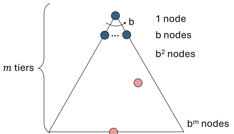
• Cartoon of search tree: $b$가 branching factor, $m$이 maximum depth
• Number of nodes in entire tree(전체 노드 수): $O(b^m)$
  

1. DFS
strategy that selects the deepest frontier node from the start node for expansion
깊이 우선 탐색. frontier에서 선택한 노드를 끝장을 본다고 생각하자.
즉, 가장 깊은 frontier node부터 탐색하는 전략이다.
LIFO(Last-In-First-Out) 특성을 나타내는 stack으로 표현한다.

DFS의 특성

• infinite or finite(유한할 수도, 무한할 수도 있음)
• 만약, 유한하다면, $O(b^m)$의 시간복잡도를 가짐
• 탐색 경로상의 sibling node들만 프론티어에 저장되므로, 공간복잡도는 $O(bm)$
• m이 infinite일 수 있기 때문에, completeness를 만족하지 않는다.
• 보통은 leftmost의 해가 선택되기 때문에, 깊이나 비용 상관없이 해를 찾는다. 따라서, optimality를 만족하지 않는다.

2. BFS
startegy that selects shallowest frontier node first
너비 우선 탐색. 가장 얕은 frontier node부터 탐색하는 전략이다.
FIFO(First-In First-Out)의 자료구조인 queue를 통해 구현한다.
가장 얕은 위치에 존재하는 해의 깊이를 s라고 할 때, 시간복잡도는 $O(b^s)$이고,
프론티어가 가지는 공간복잡도는 러프하게 $O(b^s)$를 가진다.

BFS의 특성

• s는 해가 존재한다면 유한하기 때문에, completeness를 만족한다.
• 만약 모든 cost가 1이라면 optimality를 만족하나, 아니라면 만족하지 않는다.

BFS vs. DFS
일반적으로, completeness와 optimality를 만족할 수 있는 BFS를 선택하나,
공간복잡도가 중요한 경우, 즉, 프론티어가 가질 수 있는 메모리 공간에 대한 부분이 더 중요한 상황에는 $O(bm)$의 공간복잡도를 가지는 DFS를 선택한다.

Iterative Deepening
DFS의 공간복잡도에 대한 이점과 BFS의 시간복잡도에 대한 이점을 동시에 취하고 싶다는 아이디어에서 출발해, depth level을 정하고 반복적으로 DFS를 취하는 방식이다.

1. 깊이 0으로 설정하고, 루트 노드만 탐색합니다. (해가 아니면 다음으로)
2. 깊이 1로 설정하고, 루트부터 깊이 1까지의 모든 노드를 깊이 우선 방식으로 탐색합니다. (해가 아니면 다음으로)
3. 깊이 2로 설정하고, 루트부터 깊이 2까지의 모든 노드를 다시 처음부터 탐색합니다. (해가 아니면 다음으로)
4. … 이 과정을 해를 찾을 때까지 최대 깊이를 1씩 늘리며 계속 반복합니다.

• 기존 DFS에서 개선되어 Completeness를 만족하고, 비용이 모두 1인 경우 최단 경로 해를 보장하기에 Optimality를 만족한다는 장점을 제공한다.
• 뿐만 아니라, 기존 BFS는 $O(b^m)$라는 형편없는 공간복잡도를 가졌지만, DFS처럼 다항 공간복잡도를 가진다.

Cost-Sensitive Search
BFS는 가장 짧은 경로를 찾아내는 건 맞지만, least-cost를 보장하진 않는다.
이를 해결하기 위해, UCS를 도입한다.

3. UCS
알고리즘에서 배웠던 다익스트라 알고리즘과 본질적으로 같은 로직이고, 알고리즘이다.
Expand the cheapest node first: 가장 비용이 싼 노드로 움직이는 경로를 탐색 plan으로 잡는 전략이다.
일반적으로 우선순위 큐를 통해 구현한다. 이때, 우선순위에 대한 기준은 cumulative cost, 누적된 비용 합이다.

UCS의 특성

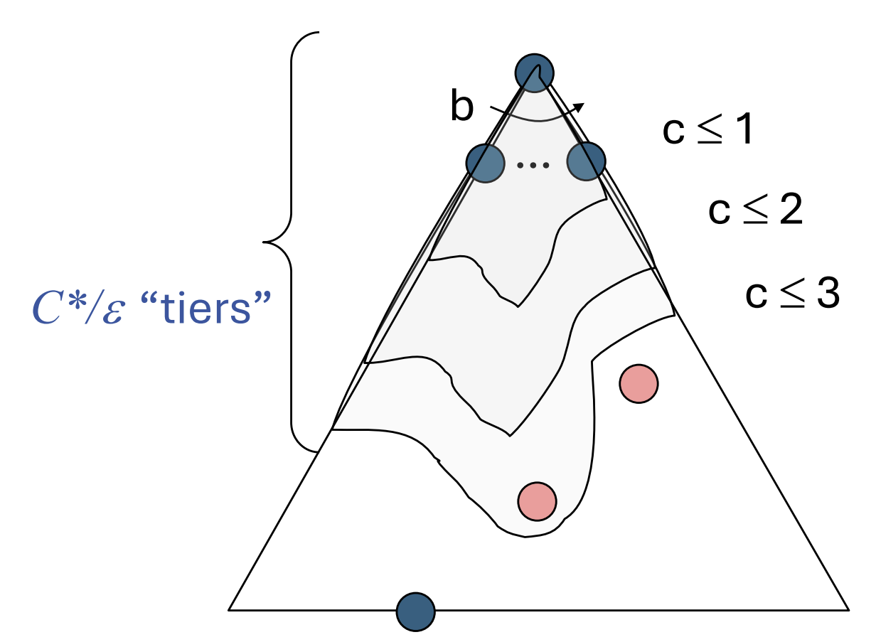
• cheapest solution보다 cost가 낮은 모든 노드들을 처리
• solution cost: $C$, minimal cost per depth: $\varepsilon$ 일 때, 탐색 깊이를 비용 관점에서 환산한 effective depth는 대략 $C/\varepsilon$이다.
• 시간복잡도: $O(b^{C*/\varepsilon})$
• 공간복잡도: $O(b^{C*/\varepsilon})$ (탐색 거의 끝날 때쯤, 프론티어에 마지막 계층의 노드들이 대부분 담겨있기 때문)
• Completeness 만족(반드시 해를 찾음. 단, C*가 유한한 값이어야 하며, negative cost가 없어야 함)
• Optimality 만족(최소 비용의 해를 찾기 때문)

DFS/BFS와 UCS
completeness와 optimality를 만족하기 때문에 장점을 가지지만,
모든 방향에 대한 옵션을 탐색하고, uninformed search에 불리하다는 단점이 있다.

따라서, informed search를 통해서 이 단점을 보완한다.

앞서 살펴본 세 가지 탐색 알고리즘(DFS/BFS/UCS)는 모두 동일하다, 단지 프론티어가 어떻게 확장되는지(그에 따른 구현 자료구조도 다름)가 다르다.
cf. 개념적으로는 모두 priority queue로 구현 가능하지만, log n 오버헤드를 피하기 위해, DFS/BFS는 각각 stack/queue를 사용함.